Locking Down on Volatility Part II

-Brian Proferes

In the previous paper we examined the mathematical definition of volatility and explored factors that can generate higher volatility in markets. In the finance world, volatility is critical in understanding financial options, and this paper will look at volatility in a more abstract manner as it pertains to call and put options. The reader should have a general understanding of options. It is recommended that any reader not previously exposed to options should gain some background knowledge to most effectively understand the article’s content.

Implied Volatility

In the previous paper we focused on looking back at a stock’s returns to calculate its volatility, but the intelligent investor will note that extrapolating past results into the future is not a recipe for sustained success. Through evaluating the prices of options, one can use mathematical formulas to come to a level of volatility implied by the price of the option. The price of an option is contingent on several factors: the underlying price, the strike price, the number of days until expiration, the current interest rate, the stock’s dividend yield, and of course the stock’s volatility. All of the listed values, except for volatility, can be known with near certainty. Although we calculated historical volatility in the previous article, volatility does not remain constant and is subject to change in the future. One could use the historical volatility as a rough estimate for implied volatility, but it is unwise to use the historical volatility in the equation that determines the option’s price. Because the forces of supply and demand influence an option’s price, we can estimate a stock’s implied volatility is through first observing the price that the option is trading for on the market given all of the known variables described above. Then we can plug all of the values in an options pricing model and solve for volatility. For example, if we observe a call option on Stock ABC with the following characteristics

● Current Underlying Price: $100

● Strike Price: $110

● Days Until Expiration: 30

● Market Interest Rate: 5%

● ABC’s Dividend Yield: 1%

● Market Price of the Option: $2

(Calculator courtesy of www.option-price.com)

We can use that information, plug it into a sophisticated option pricing model, and solve for volatility. In this case the volatility turns out to be approximately 46.25%. This implied volatility value represents the projected standard deviation of the stock’s returns over the next year. At first glance this may seem high, but remember that the option expires in 30 days and thus it must be very volatile to gain 12% to just finish at the money. If we increase the number of days to 100, then the implied volatility drops to 24.25%; an increase to 365 days will produce an IV of 10.43%, which is in line with our intuition. How will changes in the option’s price impact the implied volatility? Let’s say there is greater demand for this option and so its price is now $5. An investor who is paying $5 on a call option that is already $10 out of the money, with all else equal, must expect the stock will be more volatile than it would be if it were only selling for $2! In the previous example the stock only had to reach $112 for the investor to break even (For calls, the strike price plus option price is the breakeven value), but now, under the same conditions, the stock must reach $115 to break even. In other words, investors believe the stock is going to be more volatile and will be able to cross the strike price; therefore, they will pay more money for the option. Remember that there is another side to the transaction: If the seller of a call option expects a stock to be volatile, then he or she will want to be compensated more for assuming a greater amount of risk. We can thus conclude that in general there is a positive relationship between the price of an option and implied volatility: if an investor believes a stock will be more volatile in the future, they will pay more for the option, thus increasing the option’s price and its implied volatility.

Implied Volatility Skew

One important question the intelligent investor may ask is: If I have a call option that is currently $5.00 out of the money, and also a put option similarly $5.00 out of the money, will they be priced the same? This question is equivalent to saying: Given a stock with a current underlying price of $100, will a call option with strike price of $105 have the same price as a put option with strike price of $95? In order words, will volatility be constant whether or not the market rises or falls? Recall from the last paper we described how markets tend to be more volatile when they fall than when they rise. However prior to the market crash of 1987, the general outlook in the market was that volatility was constant, that is, the call option and the put option described above would be priced about the same. Remember that the buyer of an option can only realize a maximum loss of the price they paid for the option; the sellers could suffer serious losses if they sell a put that goes to zero or theoretically infinite losses if they sell a call option. When you sell an out of the money put option, you are hoping the market will either remain as is or increase. The opposite holds for selling an out of the money call option: you hope the market will either dip or stay constant. Given that the market will tend to drop faster than it will rise, with all else equal, a seller of a put option will want to demand greater premium than if they were selling a call option. This results in the presence of an implied volatility skew: where puts and calls with strike prices equidistant to the underlying will trade at different implied volatilities. Often times the put will trade with higher implied volatility and thus at a higher price.

Another way to conceptualize the concept of volatility skew is to first make the assumption that a majority of the investors in the stock market are long, which means they benefit when prices increase. Any wise investment firm will want to hedge against potential losses, and that hedging can be achieved through both buying puts or selling calls. If you buy a put, or sell a call, you benefit in the event of a market downturn; thus they serve as instruments that minimize losses when their main investments flounder. Simple rules of supply and demand will state that the increased demand for downside puts, and decreased demand for upside calls, will result in the price of puts increasing, and the price of calls decreasing. When prices rise, so does implied volatility. The following graph, from the book Exotic Options and Hybrids, demonstrates this principle:

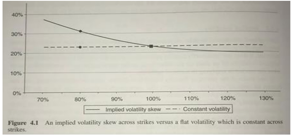
The straight dotted line shows volatility that is constant throughout strike prices, which is the assumption made in the famous Black Scholes option valuation equation. It is one of the model’s shortcomings, and traders can capitalize on the discrepancies in prices if there is significant volatility skew present. A misconception that the reader should not make is that based on the increasing skew, prices for far out of the money puts must be higher than those near the money; this notion is incorrect.

(Graph courtesy of dough.com)

Although we described the relationship between implied volatility and price as positive, one must not forget that implied volatility is derived through plugging all known numbers into an equation and back solving for volatility; option models aren’t linear and thus small increases in prices for far out of the money puts will have a greater impact on the implied volatility than small increases in the price for near the money puts. The graph to the left, which shows the price of the option, clarifies this possible misinterpretation.

Other Volatility Skews

The volatility skew generally observed is the one described above, but there are some cases that can deviate from the norm. For instance, what if there is a strong bull market that prompts a high demand for call options? The result is an inverted skew, where out of the money calls are more expensive than similarly out of the money puts. I magine an upward sloping line in the graph to reflect this reverse skew. This situation could occur if there is a rapid gain in a market, and those who are selling call options see the strong rise as a sign that they deserve a greater risk premium and thus they will charge more for the call option. Biotech stocks, newly issued companies, or commodities may be subject to this type of skew. Another volatility phenomena is a volatility smile. The graph will take a parabolic, or smile shape. Out of the money options have a greater implied volatility than near the money options. Thus there is greater market demand for options that are either well in or out of the money. Such could be the case when investors are hedging against large market swings or unforseen “black swan” events.

Investors may be both hedging against large losses and purchasing cheaper out of the money calls that would benefit in the event of a large market surge. The following graph, courtesy of theoptionsguide.com, shows the idea of volatility smile.

Conclusions

Understanding volatility is paramount if one wants to dive into derivatives, specifically options. We introduced the idea of implied volatility and contrasted it to realized or historical volatility. A brief analysis showed a positive relationship between an option’s price and its implied volatility, but the caveat was issued that just because an option has a higher implied volatility than another does not necessarily mean it is more expensive. The idea of implied volatility skew was derived and several types of observed skew were described to account for the most likely market environments.

Works Cited:

Bouzoubaa, Mohamed, and Adel Osseiran. Exotic Options and Hybrids: a Guide to Structuring, Pricing and Trading. John Wiley & Sons, 2011.

“What Is Volatility Skew? | Everything You Need to Know.” The Dough Blog, www.dough.com/blog/volatility-skew.